|
|
This document begins by explaining why we thought a W8LD downfill cabinet would be a useful addition to the range, through the use of ViewPoint software and direct sound field predictions in MATLAB. Having made the case for the product, a modeling strategy is described which allows for quick estimation of the most important parameters. As an initial verification these parameters are used in a refined model which includes the specific design of the acoustic devices. Integration with the main line array and determination of transfer functions required for the downfill cabinet are performed with this model.
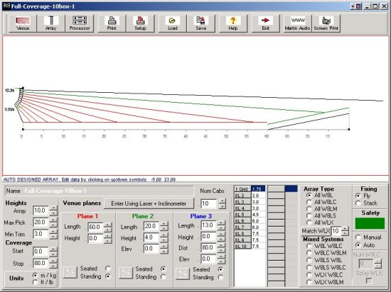
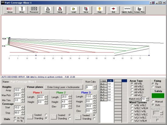
Throughout this document we will be considering 2 different arrays in the same venue, one using 10 the other using 8 W8L cabinets. The 10 box array is required to cover the entire venue whilst the 8 box array is only required to cover from 15m out. A ViewPoint entry screen of both these arrays isshown in Figs (1 and 2).
Merely looking at the aiming of the elements gives us an indication of the relative performance of the arrays, however, we can examine this more closely. The current state of our MATLAB based soundfield model enables the band averaged pressure distribution to be calculated from source data originating from:
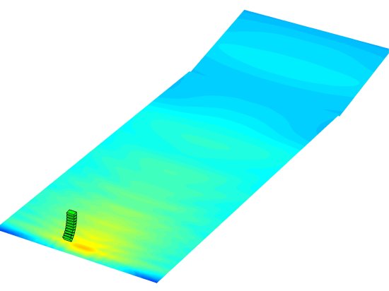
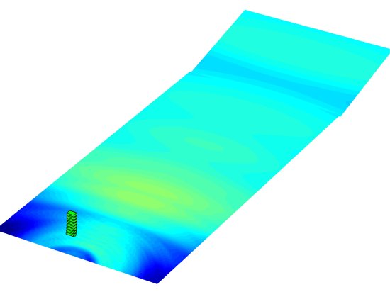
Different types of source characterisation can easily be combined within one model, this will be shown to be useful later. To view the performance of the above arrays, however, a level 3 model is used with all radiating elements (3 HF Horns per box) driven equally.
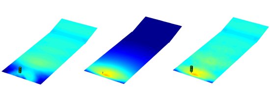
Figs (3,4,5,6) show each array at 3150Hz and 8000Hz. Performance is as expected, coverage start is well defined in both setups with the 8 box partial coverage system producing a louder and more even pressure distribution within its coverage limits.
So, assuming we can engineer one or two devices to cover from just below the array to the coverage start of the main system, we will have achieved a more efficiently utilised and balanced system without changing the overall extent of the array. In order for a one box system to achieve even coverage, output from the lower boxes is attenuated and upper box output is boosted. Using a downfill reduces the magnitude of this eq and allows more elements to contribute to the furthest positions, thus providing the system with more headroom and more HF throw. Figs (7 and 8) show the output from the lowest 5 boxes demonstrating the relatively expensive use of elements for such a small region of coverage.
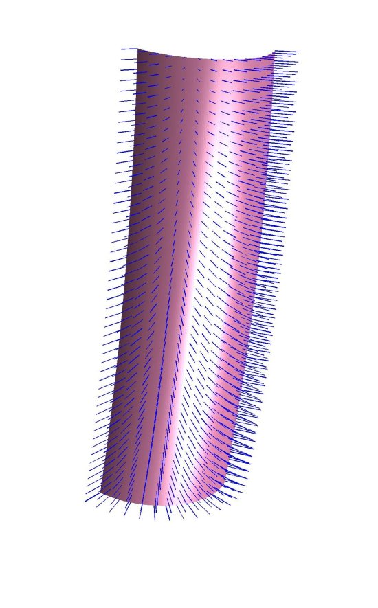
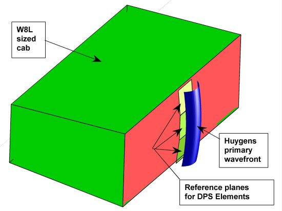
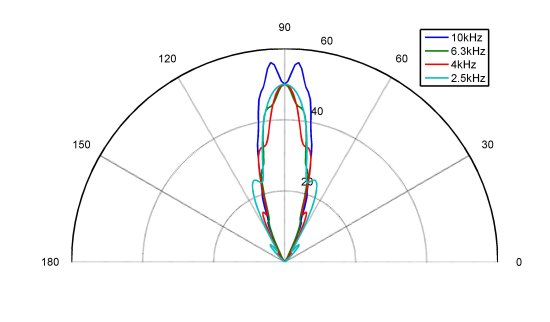
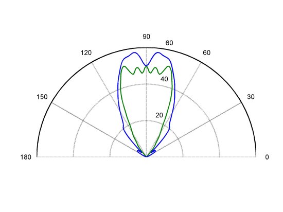
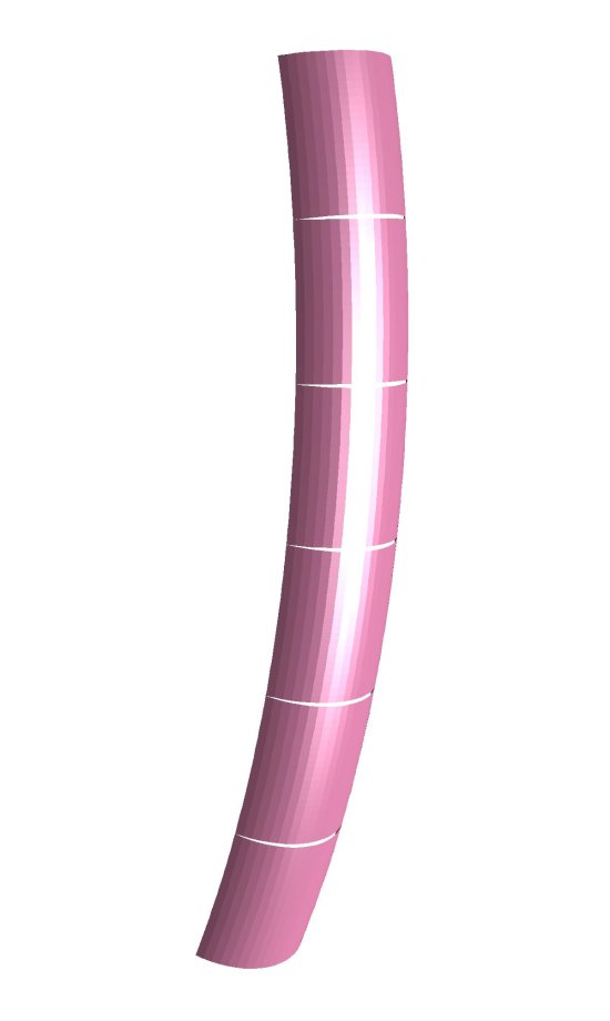
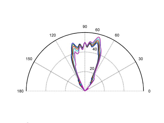
In order to get a reasonable approximation of the radiation from an idealised wavefront shape we need to revert back to a level 2 source; the Huygens wavelet. During the initial design of the W8L a 2D Huygens wavelet model was formulated and showed usefully good agreement with measured data. This model has developed into a somewhat more sophisticated 3D one with an extremely flexible method for defining the primary wavefront in the form of a Coons surface (a surface defined by the bilinear blending of boundary curves which are in fact NURBS curves). For the purposes of this investigation we are content to define the surface by boundary arcs, included angles 20 deg vertical by 120 deg horizontal as displayed in Fig (9) and in contextin (10). The vertical polar at 10m of this source is shown in fig (11)
The polars indicate that a simple uniformly driven arc source is perhaps not the most ideal arrangement at the highest frequencies. It should also be noted here that the higher frequency polars are very sensitive to measurement distance since we are assessing a sound source of dimensions significantly larger than the wavelength at the higher frequencies. This issue will be revisited later but for now the uniformly driven arc is a good starting point.
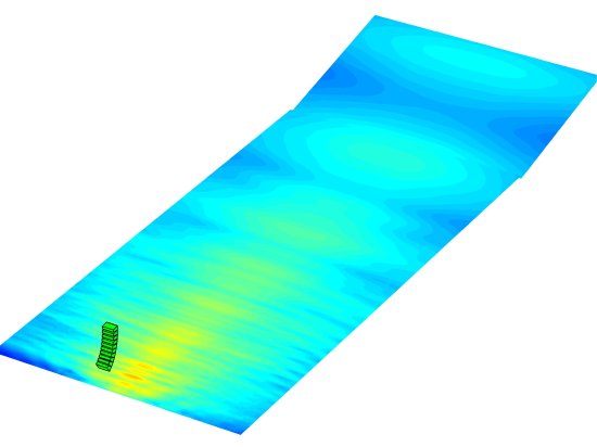
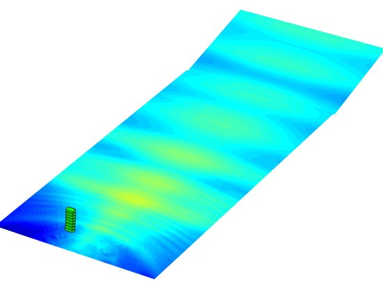
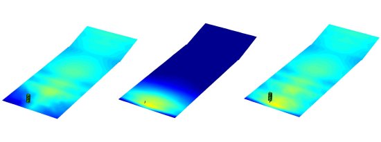
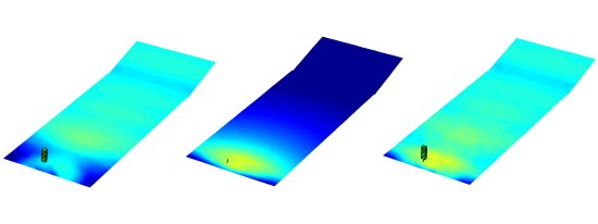
Using the idealised arc shaped wavefront and the level 3 based data of the partial coverage system from earlier, we can assess the performance of a combined system. Two arc wavefronts are positioned under the main array splayed at 20 deg to each other, the top wavefront is angled at 11.75 deg to the main array. Some very simple eq has been applied to the main array in the form of a gain reduction to the last 2 cabinets of the main array, smoothing out the SPL in the downfill transition region. Fig (12,13) shows the individual output of the sub-arrays and the combined systems at the same two 1/3 oct band frequencies of 3.15kHz and 8kHz. The combined plots indicate good integration with very little destructive interference between the systems.
The overall level of the downfill system has been adjusted to fill in the gaps in coverage of the line system at the edges of the venue in the transition region. This has resulted in system that quite an intense hot spot just in front of the array, we address this in the next section where we seek to approximate the idealised wavefront with horn devices.
|
|
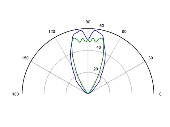
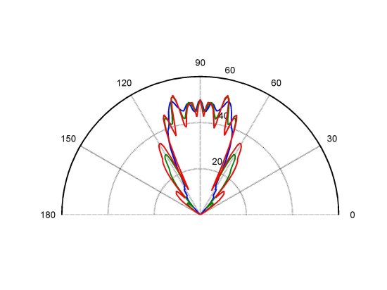
Having established the viability of the 20 deg curved wavefront as a suitable downfill we now need a physical implementation. If we took the ideal wavefront and split it into 3 sub wavefronts each of which was the output from a horn device, we would expect very similar output to the ideal providing the sub-wavefronts were correctly shaped. This easy is to check, Fig (14) shows the 10m 1/3 oct polars of the 2 ideal wavefronts at 3.15khz and 8kHz and Fig()is the equivalent polar using 6 wavefronts as depicted in Fig (16)
|
|
|
|
As expected the two polars are virtually identical. It is interesting at this point to investigate the effect of an improper wavefront shape. Fig(17) displays the effect of increasing the vertical wavefront curvature, pronounced side lobes and a more ragged response within the coverage cone are apparent. The techniques employed to realise the prescribed vertical wavefront shape and addition innovation applied to improve horizontal dispersion can not be disclosed at this stage.
|
|
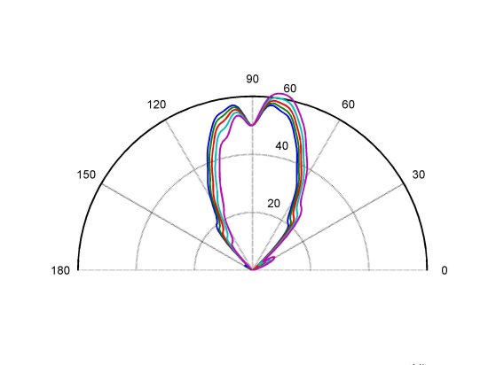
In the last section we discovered that in order to integrate well, the output within the first ten meters of the downfill section was too loud. Subdividing the wavefront provides the opportunity of producing an asymmetric vertical response by changing the gain to each HF horn. Figs(18,19) show how varying the gain effects the vertical 10m polars. The top horn always receives the full input power with the rest of the horns receiving powers proportional to how far it is away from the last horn and a constant factor. Changing the constant factor alters the rate of power decay from top to bottom horn. We can see that the range of manipulation is considerably wide and well behaved.
|
|
|
|
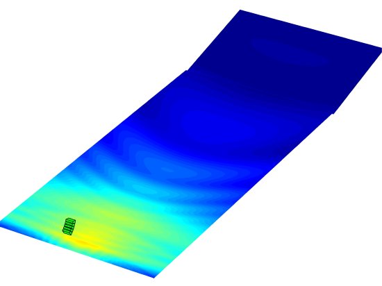
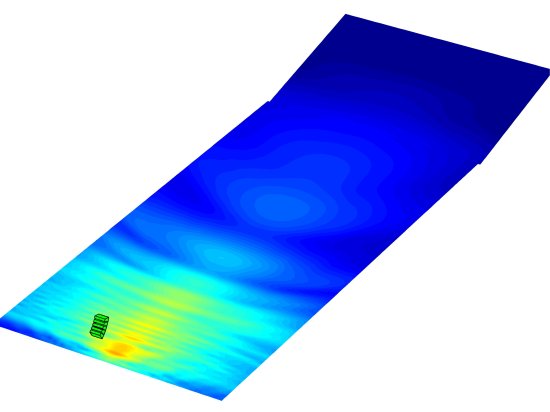
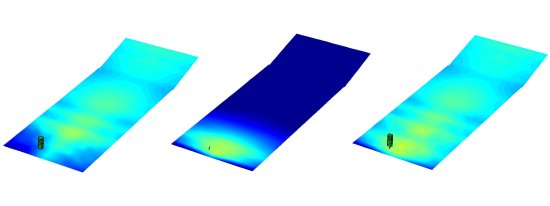
With a suitable gain distribution selected, we can see the results in the venue in Fig(20,21). The output within the downfill coverage region is now more even and better matched to that of the line array coverage. In practice the gain distribution is achieved passively with resistor networks, each W8LD has a switch which sets the box in either upper or lower mode, hence, no additional amplifier channels are required.
|
|
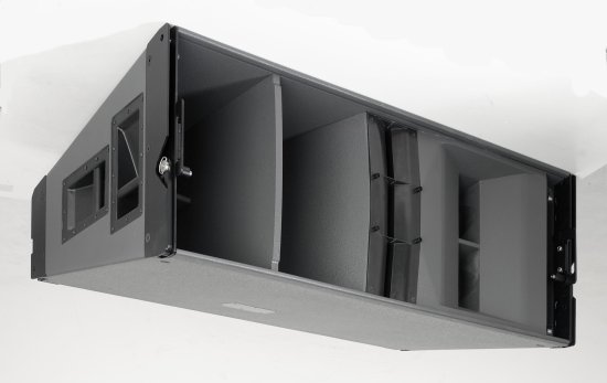
Finally a view of the finished product complete with mid an lf horns is shown in Fig(22). ViewPoint support for the W8LD is available immediately (version 3.06) with DISPLAY following soon.
Through the use of a blend of modelling techniques such as Huygens wavelet and boundary element analysis a specification for the acoustic performance of the W8LD was determined and various assumptions were tested. Acoustic devices were designed to meet this specification and their performance was correlated with the expected output.
Using one or two W8LD cabinets for the first 10-20m of coverage allows the W8L system to be much less curved and this significantly increases throw and headroom in the region beyond that of the downfill elements. Replacing one or two W8L cabinets with the same number of W8LDs gives superior performance over the whole coverage region. Additionally, the higher an array is flown, the more curved it becomes and the array curvature reduction generated by using W8LDs is particularly beneficial in this situation.
It is not advisable to reduce the W8L count further as shorter line arrays have reduced vertical pattern control in the low frequency range and therefore excite room modes and reverberation more. Replacing, say, four W8Ls with the same number of W8LDs is not optimal in most situations either. The 20 vertical dispersion means the upper W8LDs cover out to 60m or more at which distance the use of W8L line array elements is far more appropriate.